Weeding out the competition

I may be a little late to the game on this one, but a few months ago there was some controversy surrounding Saskatchewan’s cannabis licensing lottery, where several businesses won multiple permits across the province despite a large number of applicants in each municipality. One cannabis company, Prairie Sky Cannabis, was able to obtain four permits: one in each of Battleford, Estevan, Martensville and Moosomin. An article in the Leader Post claimed the probability of this happening was only 1 in 1.3 million!

Only one permit was up for grabs in each of the four communities, and the number of applicants was 20 in Battleford, 54 in Estevan, 47 in Martensville, and 26 in Moosomin. So the probability of getting four permits was calculated as:

(¹⁄₂₀)*(¹⁄₅₄)*(¹⁄₄₇)*(¹⁄₂₆) = ¹⁄_1319760.

But hold on a second! This would be the probability of getting those four permits if they had only applied in those four communities. In fact, Prairie Sky applied in all 32 communities! So the probability calculation should consider the probability of getting four or more permits in any set of communities. There are 35,960 different ways that Prairie Sky could have won 4 permits.

Calculating the probability

Since the number of available permits and number of applicants differs between communities, the probability calculation is quite difficult. To make things easier, I simply run a simulated lottery 10,000 times and see how often Prairie Sky wins four or more permits. The dataset is shown below, and is accessible in .csv format on my Github page. Code for the R analysis I perform here is also available in that repository.

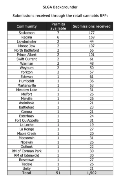
The numbers here don’t exactly match the ones reported in the Leader Post article, as presumably some of the applicants withdrew or were removed from the lottery. However, I can still illustrate the general idea using these numbers. I also assume that an applicant could only obtain a single permit in each community, regardless of the number of permits available. Let’s read in the data.

c.data <- read.csv("sk_cannabis_data.csv", row.names = 1)
n <- NROW(c.data)

I replicate the original (incorrect) calculation using the new numbers:

# Calculate probability of getting a permit in each city
permit.prob <- c.data$permits/c.data$submissions
names(permit.prob) <- rownames(c.data)
cities <- c("Battleford", "Estevan", 
       	"Martensville", "Moosomin")
ps.prob <- prod(permit.prob[cities])
ps.prob
# [1] 4.338152e-07

The probability is very small: 4.34x10^-7. Now, I perform the simulation to get the correct probability that assumes the applicant has applied in all 32 communities. This is simply drawing samples from a Bernoulli distribution in each community and seeing how many permits were won. I run 10,000 replications of this simulation.

n.sim <- 10000
n.permit <- rep(0, n.sim)

for (i in 1:n.sim) {
  np.obtained <- rbinom(n, rep(1, n), permit.prob)
  n.permit[i] <- sum(np.obtained)
}

The estimated probability is then the proportion of simulations resulting in four or more permits.

# Prob of getting 4 or more permits
mean(n.permit>=4)
# [1] 0.0287

The probability of a single applicant receiving four or more permits in any community is 2.87%. This is still a fairly small probability, but is much, much higher than what was reported in the news article. Let’s look at the distribution of the number of permits won:

library(ggplot2)

p.df <- data.frame(Permit=n.permit)
ggplot(data=p.df, aes(Permit)) + geom_histogram() +
    theme(axis.text=element_text(size=14),
      axis.title=element_text(size=14,face="bold"))

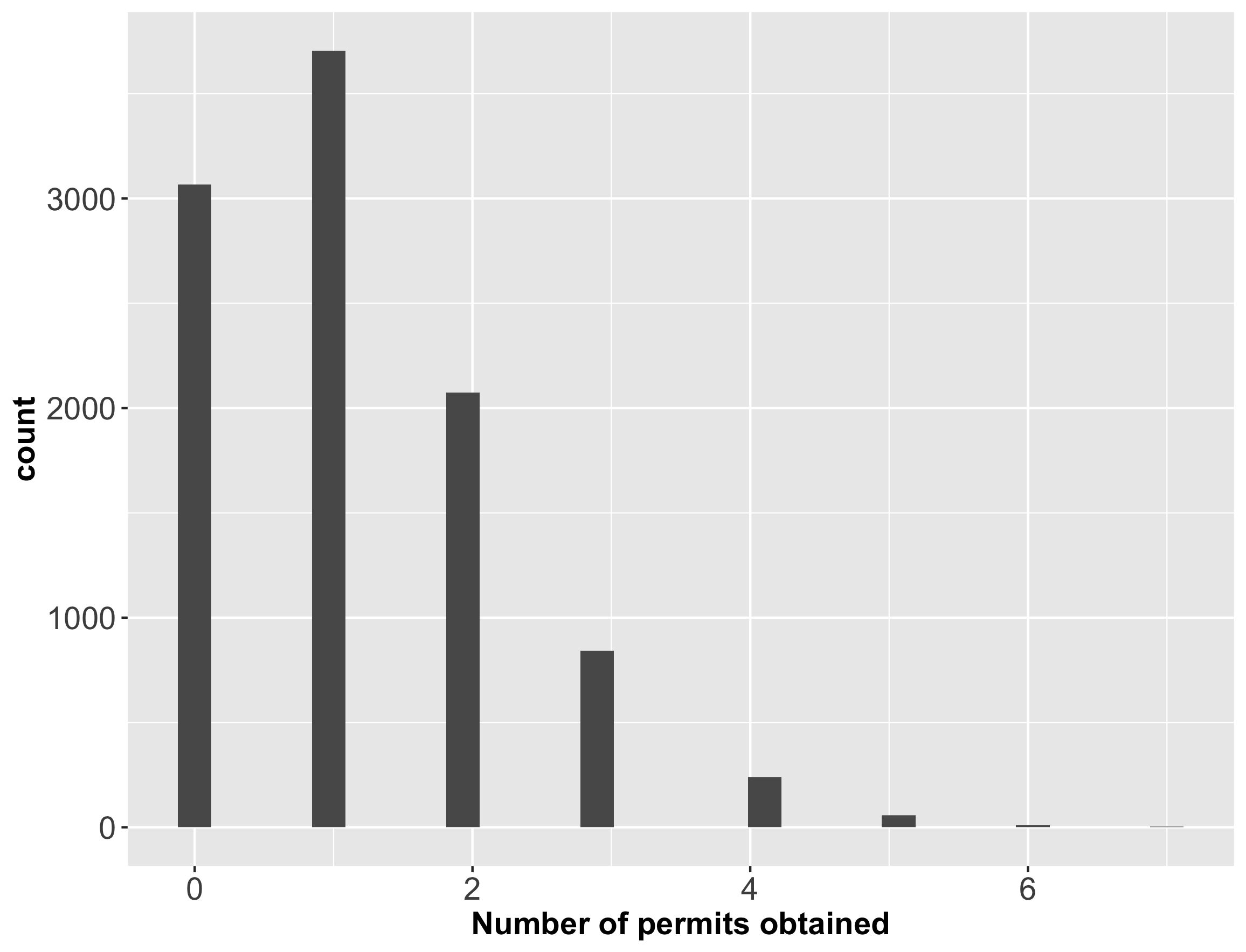
So it’s likely that a single applicant could have obtained zero, one, or two permits. However, an applicant getting four or more permits is fairly unlikely.

What if…

As mentioned above, I assumed a single applicant could win only a single permit in each community. But how would the calculation change if multiple permits could be obtained in a single community?

As it turns out, the calculation becomes much simpler. We only need to consider the total number of permits available, and the total number of applicants. Then, if an applicant applies for all possible permits, the distribution is hypergeometric! There are 51 total permits available, and the “population size” is 1502 (the number of applicants). So the distribution is:

Hypergeometric(N=1502, K=51, n=51),

where N is the population size, K is the number of “success” items in the population, and n is the number of draws from the population. I then calculate the probability using the CDF of the hypergeometric distribution:

# Calculating probability of 4 or more permits if you 
# could obtain multiple permits in each city
avail.permit <- sum(c.data$permits)
n.wo.permit <- sum(c.data$submissions) - avail.permit

# Prob of getting 4 or more permits
1-phyper(3, avail.permit, n.wo.permit, avail.permit)
# [1] 0.09116339

In this case, the probability of four or more permits is 9.1%. Out of curiosity, the N parameter in this distribution is fairly large… could I have used the binomial distribution to approximate this probability? Let’s find out:

# Would binomial have worked as well here?
1-pbinom(3, avail.permit, 
	    avail.permit/(avail.permit+n.wo.permit))
# [1] 0.09459626

The binomial calculation gives the probability at 9.4%. So the binomial distribution would have worked as well.